How to Insert a Check Mark (Tick ✓) Symbol in Excel [Quick Guide]
How to Insert a Check Mark (Tick ✓) Symbol in Excel [Quick Guide]
Check Mark Vs Check Box
While a check mark and a checkbox may look somewhat similar, these two are very different in the way it can be inserted and used in Excel.
A check mark is a symbol that you can insert in a cell (just like any text that you type). This means that when you copy the cell, you also copy the check mark and when you delete the cell, you also delete the check mark. Just like regular text, you can format it by changing the color and font size.
A checkbox, on the other hand, is an object that sits above the worksheet. So when you place a checkbox above a cell, it’s not a part of the cell but is an object that is over it. This means that if you delete the cell, the checkbox may not get deleted. Also, you can select a checkbox and drag it anywhere in the worksheet (as it’s not bound to the cell).
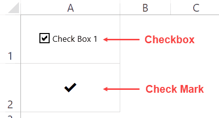
You will find checkboxes being used in interactive reports and dashboards, while a checkmark is a symbol that you may want to include as a part of the report.
In this article, I will only be covering check marks. If you want to learn more about checkbox, here is a detailed tutorial.
There are quite a few ways that you can use to insert a check mark symbol in Excel.
Inserting Check Mark Symbol in Excel
In this article, I will show you all the methods I know.
The method you use would be dependent on how you want to use the check mark in your work (as you’ll see later in this tutorial).
Let’s get started!
Copy and Paste the Check Mark
Starting with the easiest one.
Since you’re already reading this article, you can copy the below check mark and paste it in Excel.
To do this, copy the check mark and go to the cell where you want to copy it. Now either double-click on the cell or press the F2 key. This will take you to the edit mode.
✔
Simply paste the check mark (Control + V).
Once you have the check mark in Excel, you can copy it and paste it as many times as you want.
Use the Keyboard Shortcuts
For using the keyboard shortcuts, you will have to change the font of the cells to Wingdings 2 (or Wingdings based on the keyboard shortcut you’re using).
Below are the shortcuts for inserting a check mark or a cross symbol in cells. To use the below shortcuts, you need to change the font to Wingdings 2.

Below are some more keyboard shortcuts that you can use to insert check mark and cross symbols. To use the below shortcuts, you need to change the font to Wingdings (without the 2).
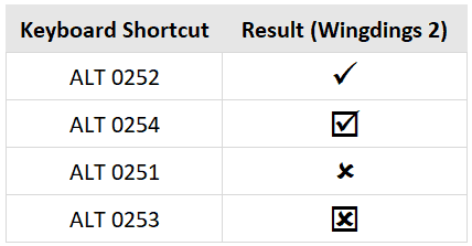
Using the Symbols Dialog Box
Another way to insert a check mark symbol (or any symbol for that matter) in Excel is using the Symbol dialog box.
Here are the steps to insert the check mark (tick mark) using the Symbol dialog box:
- Select the cell in which you want the check mark symbol.
- Click the Insert tab in the ribbon.

- Click on the Symbol icon.

- In the Symbol dialog box that opens, select ‘Segoe UI Symbol’ as the font.
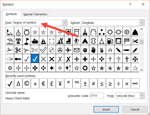
- Scroll down till you find the check mark symbol and the double click on it (or click on Insert).
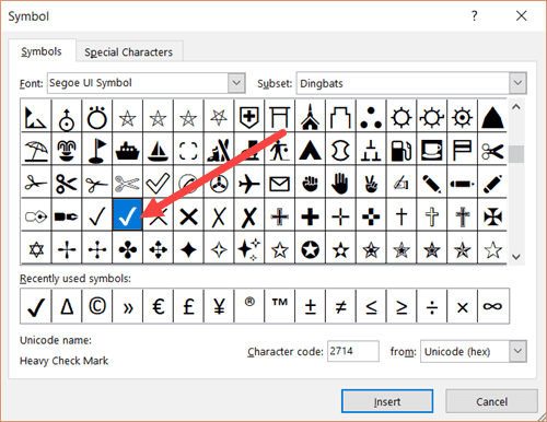
The above steps would insert one check mark in the selected cell.
If you want more, simply copy the already inserted one and use it.
Note that using ‘Segoe UI Symbol’ allows you to use the check mark in any regularly used font in Excel (such as Arial, Time Now, Calibri, or Verdana). The shape and size may adjust a little based on the font. This also means that you can have text/number along with the check mark in the same cell.
Using the CHAR Formula
You can use the CHAR function to return a check mark (or a cross mark).
The below formula would return a check mark symbol in the cell.
=CHAR(252)
For this to work, you need to convert the font to Wingdings
Why?
Because when you use the CHAR(252) formula, it would give you the ANSI character (ü), and then when you change the font to Wingdings, it is converted to a check mark.
You can use similar CHAR formulas (with different code number) to get another format of the check mark or the cross mark.
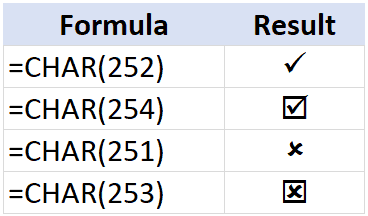
The real benefit of using a formula is when you use it with other formulas and return the check mark or the cross mark as the result.
For example, suppose you have a dataset as shown below:
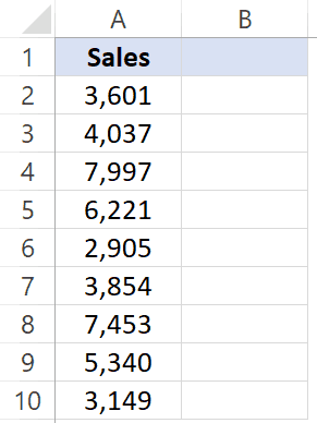
You can use the below IF formula to get a check mark if the sale value is more than 5000 and a cross mark if it’s less than 5000.
=IF(A2>5000,CHAR(252),CHAR(251))
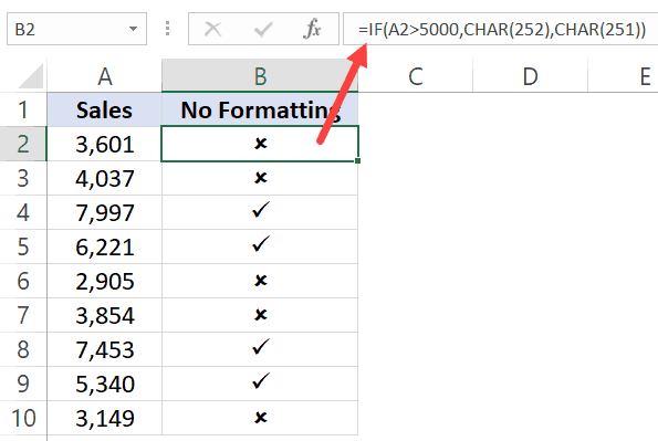
Remember, you need to convert the column font to Wingdings.
This helps you make your reports a little more visual. It also works well with printed reports.
If you want to remove the formula and only keep the values, copy the cell and paste it as value (right-click and choose the Paste Special and then click on Paste and Values icon).
Using Autocorrect
Excel has a feature where it can autocorrect misspelled words automatically.
For example, type the word ‘bcak’ in a cell in Excel and see what happens. It will automatically correct it to the word ‘back’.
This happens as there is already a pre-made list of expected misspelled words you’re likely to type and Excel automatically corrects it for you.
Here are the steps to use autocorrect to insert the delta symbol:
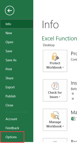
- Click on the File tab.
- Click on Options.
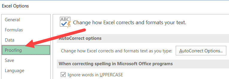
- In the Options dialogue box, select Proofing.
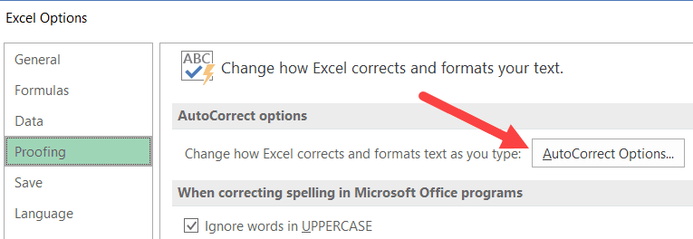
- Click on the ‘AutoCorrect Options’ button.
- In the Autocorrect dialogue box, enter the following:
- Replace: CMARK
- With: ✔ (you can copy and paste this)

- Click Add and then OK.
Now whenever you type the words CMARK in a cell in Excel, it will automatically change it to a check mark.
Here are a few things you need to know when using the Autocorrect method:
- This is case sensitive. So if you enter ‘cmark’, it will not get converted into the check mark symbol. You need to enter CMARK.
- This change also gets applied to all the other Microsoft applications (MS Word, PowerPoint, etc.). So be cautious and choose the keyword that you are highly unlikely to use in any other application.
- If there is any text/number before/after CMARK, it will not be converted to the check mark symbol. For example, ‘38%CMARK’ will not get converted, however, ‘38% CMARK’ will get converted to ‘38% ✔’
Related Tutorial: Excel Autocorrect
Using Conditional Formatting to Insert Check Mark
You can use conditional formatting to insert a check mark or a cross mark based on the cell value.
For example, suppose you have the data set as shown below and you want to insert a check mark if the value is more than 5000 and a cross mark if it’s less than 5000.

Here are the steps to do this using conditional formatting:
- In cell B2, enter =A2, and then copy this formula for all cells. This will make sure that now you have the same value in the adjacent cell and if you change the value in column A, it’s automatically changed in column B.

- Select all the cells in column B (in which you want to insert the check mark).
- Click the Home tab.
- Click on Conditional Formatting.
- Click on New Rule.

- In the ‘New Formatting Rule’ dialog box, click on the ‘Format Style’ drop down and click on ‘Icon Sets’.

- In the ‘Icon Style’ drop-down, select the style with the check mark and cross mark.

- Check the ‘Show Icon only’ box. This will ensure that only the icons are visible and the numbers are hidden.

- In the Icon settings. change the ‘percent’ to the ‘number’ and make the settings as shown below.

- Click OK.
The above steps will insert a green check mark whenever the value is more than or equal to 5000 and a red cross mark whenever the value is less than 5000.
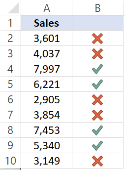
In this case, I have only used these two icons, but you can also use the yellow exclamation mark as well if you want.
Using a Double-Click (uses VBA)
With a little bit of VBA code, you can create an awesome functionality – where it inserts a check mark as soon as you double click on a cell, and removes it if you double click again.
Something as shown below (the red ripple indicates a double click):
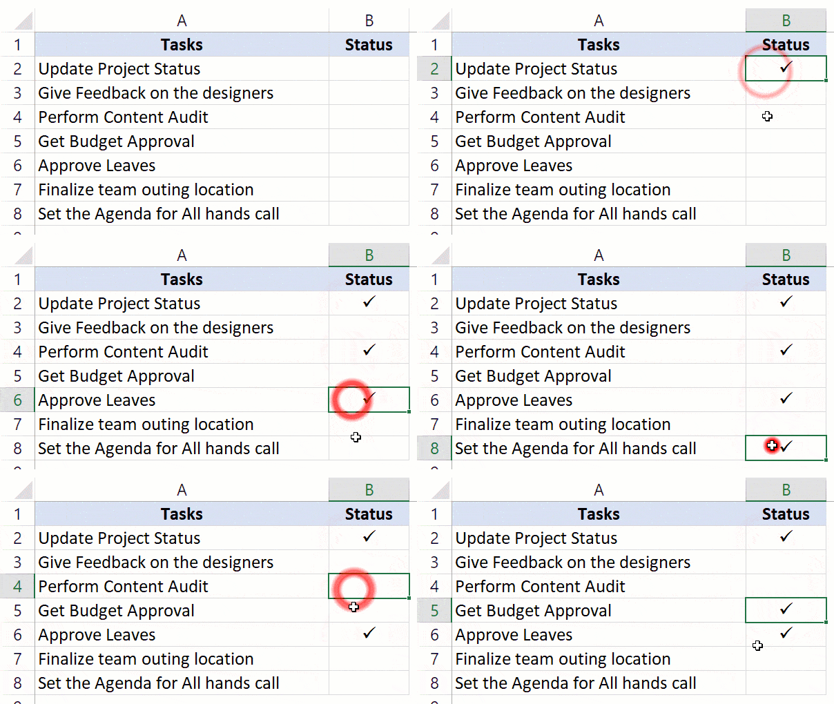
To do this, you need to use the VBA double-click event and a simple VBA code.
But before I give you the full code to enable double click, let me quickly explain what how VBA can insert a check mark. The below code would insert a check mark in cell A1 and change the font to Wingdings to make sure you see the check symbol.
Sub InsertCheckMark()
Range("A1").Font.Name = "Wingdings"
Range("A1").Value = "ü"
End Sub
Now I will use the same concept to insert a check mark on double click.
Below is the code to do this:
Private Sub Worksheet_BeforeDoubleClick(ByVal Target As Range, Cancel As Boolean)
If Target.Column = 2 Then
Cancel = True
Target.Font.Name = "Wingdings"
    If Target.Value = "" Then
        Target.Value = "ü"
    Else
        Target.Value = ""
    End If
End If
End Sub
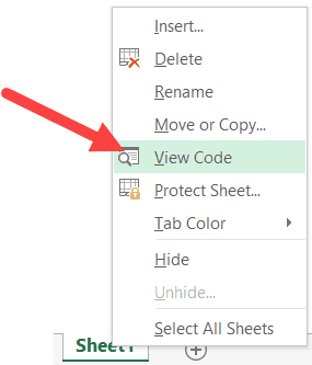
You need to copy and paste this code in the code window of the worksheet in which you need this functionality. To open the worksheet code window, left-click on the sheet name in the tabs and click on ‘View Code’
Formatting the Check Mark Symbol
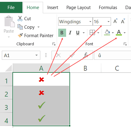
A check mark is just like any other text or symbol that you use.
This means that you can easily change its color and size.
All you need to do is select the cells that have the symbol and apply the formatting such as font size, font color, and bold etc.
Format Check Mark / Cross Mark Using Conditional Formatting
With conditional formatting, you can format the cells based on what type of symbol it has.
Below is an example: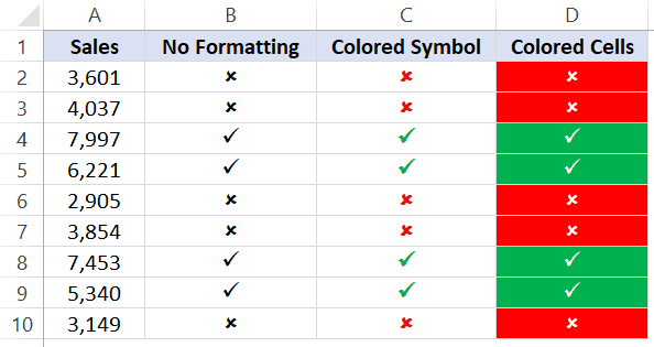

Column B uses the CHAR function to return a check mark if the value is more than 5000 and a cross mark if the value is less than 5000.
The ones in column C and D uses conditional formatting and look way better as it improves visual representation using colors.
Let’s see how you can do this.
Below is a dataset where I have used the CHAR function to get the check mark or cross mark based on the cell value.

Below are the steps to color the cells based on the symbol it has:
- Select the cells that have the check-mark/cross-mark symbols.
- Click the Home tab.
- Click on Conditional Formatting.
- Click on ‘New Rule’.

- In the New Formatting Rule dialog box, select ‘Use a formula to determine which cells to format’

- In the formula field, enter the following formula: =B2=CHAR(252)

- Click the Format button.

- In the ‘Format Cells’ dialog box, go to the Fill tab and select the green color.

- Go to the Font tab and select color as white (this is to make sure your checkmark looks nice when the cell has a green background color).

- Click OK.
After the above steps, the data is going to look as shown below. All the cells that have the check mark will be colored in green with white font.
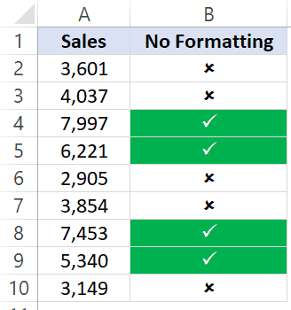
You need to repeat the same steps to now format the cells with a cross mark. Change the formula to =B2=char(251) in step 6 and formatting in step 9.
Count Check Marks
If you want to count the total number of check marks (or cross marks), you can do that using a combination of COUNTIF and CHAR.
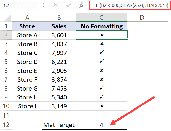
For example, suppose you have the data set as shown below and you want to find out the total number of stores that have achieved the sales target.
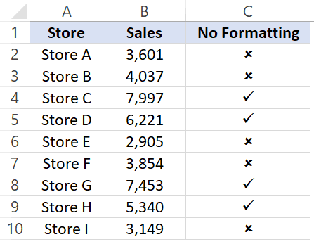
Below is the formula that will give you the total number of check marks in column C
=COUNTIF($C$2:$C$10,CHAR(252))
📤You download App EVBA.info installed directly on the latest phone here : https://www.evba.info/p/app-evbainfo-setting-for-your-phone.html?m=1


Leave a Comment